One of the key processes as an analyst while creating reports is to cleanse data from inconsistencies. Sometimes it is an item description that combines different reporting lines that need to be separated while at other times you need to convert dates formatted as text in Excel or any other platform.

What do I mean?

Improper dates in Excel would be dates that display as dates but do not behave as dates. That is, you cannot manipulate them using date functions or filter these columns using a date attribute.

Have you encountered such before?

Sometimes a system will generate dates that have a period (read full stop) as the delimiter, or a mix of dates and text dates. Other times it is the order of date parameters that makes it improper.

This article will save you loads of time that you would spend dealing with the menace and especially where you have large data sets.

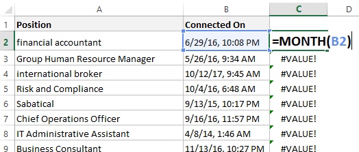
I recently downloaded my LinkedIn connections data in Excel. I have over 8,000 connections and I wanted to profile their industry and job functions. As you can see, when I tried to generate a month from the date column, I get an error.

We are going to deal with this problem right there!

Click to download the accompanying workbook.

There are a couple of ways you can convert text dates to proper dates in Excel. The 2 key methods are:

1. Using the Text-to-columns feature in Data menu
2. Combining TEXT and DATE functions

My preference is number 2 as it is scalable, that is, in case you have additional rows, you just need to auto-fill the formula.

The learning curve for this approach is not for the faint hearted.

But…

If you have had the headache of cleaning improper dates in Excel, then this is 101% worth of your time.

In this case, we want the characters before the comma formatted as a proper date where we can extract other attributes such as the day of the week (this would be more relevant for analyzing traffic of which days are people likely to be online in LinkedIn).

I shall then leave you to work on the time portion of the text string.

A date is comprised of the year, the month and the day components.

In this example, therefore, we first have to generate these three attributes as separate columns as follows.

Month attribute

In our data, the months are the digits before the first forward slash (/), right? How do we write a formula that extracts this ensuring the formula is flexible for scenarios where the day is one and two digits?

We agree on the fact that we need the first 1 or 2 digits from the left of the string. The function we shall employ here is the LEFT function.

The LEFT function extracts a specified number of characters from the left of a text string.

So we can write =LEFT (B2, 1) or =LEFT (B2, 2) for a 1 or 2 digits month attribute respectively. Is that so? Not so fast! You have 8,000 records! (I assisted one of my clients who was dealing with over 300k rows of data).

There is a logic…

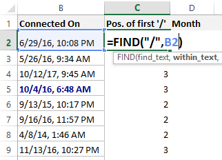
In this case, we need to use the FIND function to identify the position of the first forward slash (/). Note we have two forward slashes. We would write =FIND (“/”, B2) as shown in the diagram below.

The FIND function returns the position (a number) of a given character in a text string.

As you can see, this function will always yield a 2 or a 3.

To get the month using the LEFT function, we will always, therefore, have to know the position of the first slash (/) occurrence and then deduct one so that we do not include the slash in the final output. That is, the month will always be the digits just before the forward slash (/).

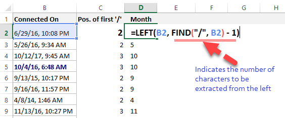
The correct (flexible for 1 or 2 digits) formula for the month attribute will therefore be as shown in the figure below.

The formula says, from the left of the text string in cell B2, extract the characters just before the first occurrence of the forward slash (as specified by the FIND function).

Day attribute

In our data, the days are the digits in between the first and the second forward slashes.

To extract the characters in between, we shall combine the MID and the FIND functions. We have already seen the use of the FIND function.

The MID function extracts a specified number of characters from a specified start position.

Syntax: This function has three parameters. In layman’s terms, we can express it as:

MID (your text, position of first character to be extracted, number of characters to be returned)

Let us go through each of this parameters.

• Your text is the improper dates in column B. in row 2, this is cell B2
• The position of the first character is the character right after the first forward slash. We shall employ the same FIND function as above, but, instead of deducting one, we shall add a one so that once the FIND function tells us the position of the first slash, we then start from the character immediately after that position. This part of the formula is:

=FIND (“/”, B2) + 1

• The number of characters to be extracted is either 1 digit or 2 digits, but how do we tell Excel to swap between 1 or 2 digits as we auto-fill the formula in the subsequent rows?

Follow along…

Mathematically, this number is expressed as:

Position of second slash – Position of first slash – 1

I hope you are able to see that from the data.

To implement this expression we need to identify the position of the second slash using the FIND function.

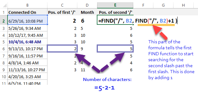
To do this, we shall nest a second FIND function within the first FIND function so that Excel is able to skip the first slash and return the position of the second slash. Take a look.

Re-writing this portion of the formula, we get:

Now that we have covered the 3 parameters, let us put them together.

The formula that will return the day attribute from the original text is therefore written as follows:

                =MID (B2, FIND (“/”, B2) +1, FIND (“/”, B2, FIND (“/”, B2) +1) – FIND (“/”, B2) – 1)

Year attribute

The two digits after the second slash are the last two digits of the year attribute.

This could be a problem if we had dates with a mix of 19xx and 20xx. Luckily, for LinkedIn the dates are in the 20xx range. As such, once we extract the 2 digits after the second slash, we shall concatenate/join this to 20.

To extract the 2 characters, we shall use the MID and FIND functions. The logic is the same as above hence I shall not go into the details.

• Formula for the 2 digits: =MID (B2, FIND (“/”, B2, FIND (“/”, B2) +1) + 1, 2)
• Year formula:                   =20 & MID (B2, FIND (“/”, B2, FIND (“/”, B2) +1) + 1, 2)

We have come a long way!

We have extracted the three attributes that make up a date. It is time now to generate a proper Excel date. To do this we use the DATE function.

This function requires us to specify the year, month and day in that order. In our example, we’ll write:

=DATE (G2, D2, F2)

If you wish to eliminate the intermediary columns so that you only have the one with proper dates, then you could re-write the DATE formula as shown below. I encourage you to always start with the intermediary steps before nesting. You can maintain these columns but hide them.

Here is the formula:

=DATE (20 & MID (B2, FIND (“/”, B2, FIND (“/”, B2) +1) + 1, 2),

                       LEFT (B2, FIND (“/”, B2) – 1),

                                   MID (B2, FIND (“/”, B2) +1, FIND (“/”, B2, FIND (“/”, B2) +1) – FIND (“/”, B2) – 1)

              )

If you master the above, you can handle literally any text string in Excel.

These are the sort of things that keep people awake at month end reporting, but, you can help me help your colleagues in similar scenarios.

Kindly click the share buttons on the left of your screen.

Let me know in the comments below other approaches that you use in similar scenarios …or a related question that you would want us to address.