Do you have data in multiple worksheets that you wish to aggregate into a single sheet? Then this article is primarily written to address just that -how to consolidate data from multiple worksheets to a summary worksheets in Excel.

Recently, I received a query from one of the people I’ve trained in Excel. This person works for an automotive industry and had an Excel file that he uses to track vehicle sales by various sales reps in the organization. He had maintained the vehicle sales for each month in a separate worksheet and sort my help to have a quarterly sales report that would update once the monthly numbers are updated.

Using the Consolidate Feature

The Consolidate Feature in MS Excel gives you two options to aggregate your data:

• Consolidate by Position
• Consolidate by Category

Both methods can also be achieved by use of a formula.

In this article, we shall focus on these two methods as well as show you how to use a formula to consolidate multiple worksheets by position.

Related:

• Use Excel macros to automate consolidation
• Combine multiple worksheets using Power Query

METHOD 1: Consolidate by Position

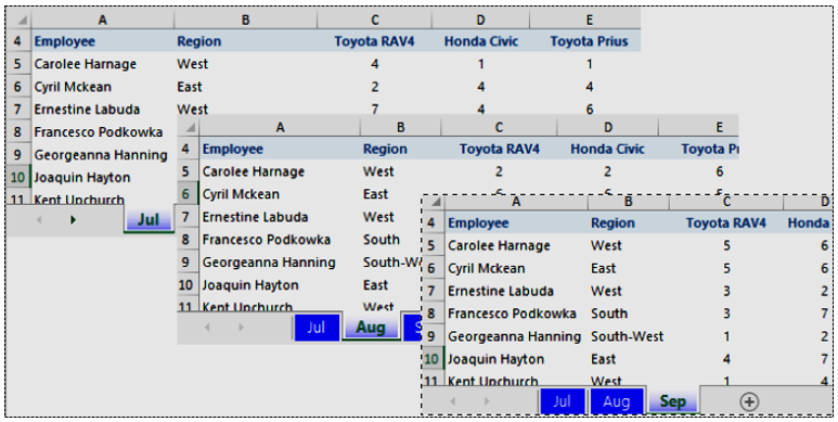
The figure below shows the sample data for Quarter 3.

STEP #1: Create the Layout for the Summary Worksheet

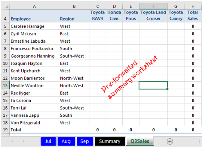
To consolidate the above, we shall create a new worksheet with a similar structure/layout with the source monthly sales worksheets. That is, the vehicle types, the employee and the region shall be pre-typed as shown below.

NOTE:

When consolidating by position, each range in the monthly sales worksheets (source data) need to have the same layout. The reason this method is referred to as Consolidate by Position is by the virtue that all the source worksheets -in this case July, August & September worksheets -have the same data structure…in the sense that cell C5, for instance, stores the sales for Carolee, for RAV4. This is consistent in all the worksheets. If this is not the case, you may need to look at the Consolidate by Category or how to use Power Query to learn how you can achieve the same results.

STEP #2: Invoke the Consolidate Feature

Select cell C5 in the summary worksheet and from the Data menu click Consolidate.

STEP #3: Set the Data Source and Base Function

When you click the Consolidate command in step 2 above, the Consolidate dialog box pops up allowing you to specify what data you want to summarize.

The default function for aggregation is the SUM function but you can change this depending on your needs.

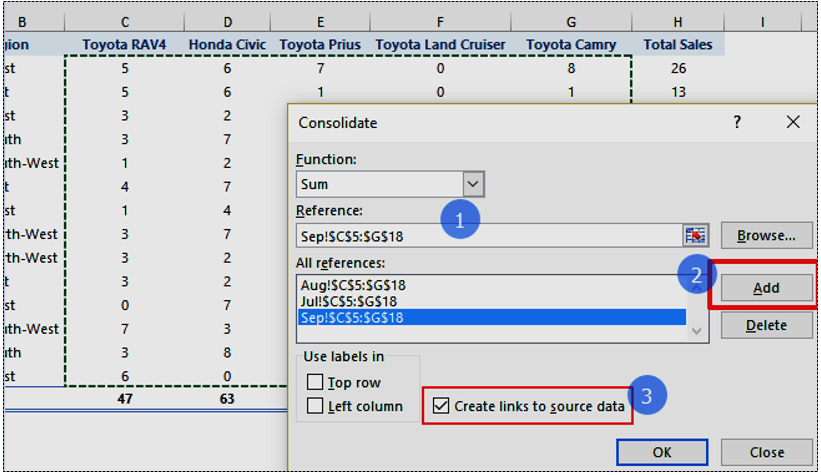
Click inside the Reference box and select the July figures. Be careful to only select the numbers without the column headings and other text. Once you select, press the Add button.

Repeat this for each of the worksheets -Aug & Sep, pressing the Add button each time. you should end up with the following.

STEP #4: Link the Summary to the Source Worksheet

Ensure to tick “Create links to source data” so that you maintain a link to the source data for refresh purposes. Press OK.

STEP #4: The Summary Worksheet

A closer look at the summary worksheet will indicate what happened.

The summary worksheet has links/formulas that refer to the source worksheets, and therefore any update that happens in any of the Jul, Aug or Sep worksheets updates in the summary. This is made possible by the fact that we checked the box against “Create links to source data” in step 3 above.

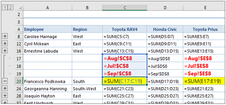
You can click on the + or – signs on the side-bar of the figure above to collapse or expand the summary.

Download the consolidate monthly vehicle sales worksheet to do it yourself.

METHOD 2: Consolidate Data From Multiple Worksheets Using a Formula

Use the file downloaded above to follow this example.

The assumption that we made in the above example about consistent arrangement and positioning holds true for this approach. It is based on the fact that a given cell, say cell C5, in all the worksheets has the same data, only that it is for different entities, in this case the different months.

STEP #1: Prepare the Summary Sheet

STEP #2: Type the Formula

In cell C5, we type the SUM function as follows…

=SUM(Jul:Sep!C5)

This step is a very critical one. To achieve this formula, once you type =SUM (…., select cell C5 in the worksheet named Jul

Immediately you select cell C5 in the Jul worksheet, hold down the SHIFT key and click the worksheet tab named Sep.

At that point, close the bracket and press enter.

What the formula says, is that sum all the cell C5’s in all the worksheets between the Jul worksheet and the Sep worksheet. That means that if you drag any other worksheet between these two worksheets, the summary sheet will also inckude the value of cells C5’s in those worksheets in the totals. It also means that if you drag out any of the worksheets in between these two worksheets, the summary worksheet will deduct the value for the removed sheet.

STEP #3: Auto-fill the Formula

The last step is to copy the formula to the other cells to get the values for the other car models and sales agents.

METHOD 3: Consolidate by Category

To consolidate by category means to rely on the column headings and/or the rows to match items.

As opposed to the consolidate by position methodology, it is not necessary to maintain consistency, that is, it isn’t mandatory to have cell C5 (as seen above) store the sales for Carolee, for RAV4. Further, the records must not necessarily be equal. That means the first sheet can have 10 records, second one 3 records, third one 7 records/rows and so forth.

The source worksheets for our example now looks like this…

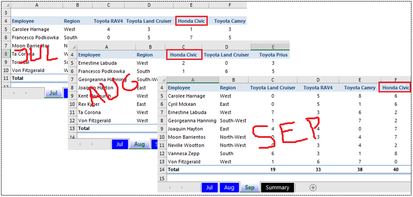
Notice, for instance, the Honda Civic model appears in different columns in each of the worksheets. Further, the number of records / rows is not uniform, as it would be the case when consolidating by position.

The steps involved are as follows:

STEP #1: Ensure the Top Rows and Left-most Columns Are Similar

For this method to work, at least the column headings as well as the items in the left-most column should be spelt the same. This is because we shall rely on these column and row labels to summarize the records.

STEP #2: Blank Summary Worksheet

In a blank worksheet that will have the summary, select a cell where you want the summary to appear. In this example, we have selected cell C5 but you can select any of the blank cells.

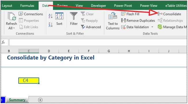
Next, click Data menu >> Consolidate.

STEP #3: Consolidate

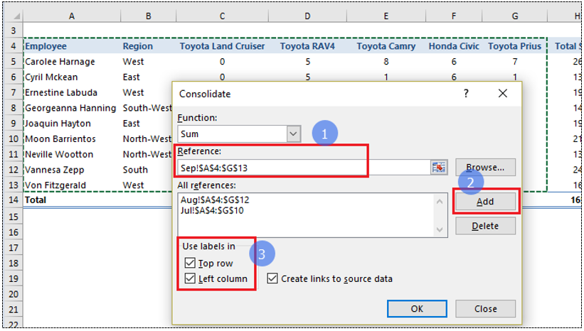
Upon pressing Consolidate from Data menu, the Consolidate dialog box pops up. Just like we did in the previous example, we shall click inside the Reference box and select, and Add the data ranges for our summary.

NOTICE in this example we select everything, including the column and row headings.

STEP #4: Use Labels for Consolidation

In step 3 above, we have selected the data including the headings. In this step, we ensure we have ticked the “Top row” and “Left column” options (see #3 in the figure above). This is where the Consolidate by Category differs with the Consolidate by Position.

Further, to create a link to the data source, we ensure we have checked the “Create links to source data” option.

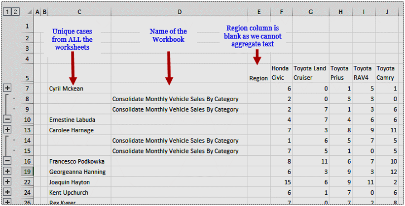
When you press OK, you will end up with a summary similar to the following:

STEP #5: The Output

The figure above shows the final summary.

As you can see, columns with text data such as the region one will not be aggregated. As such, you may have to use other formulas to lookup these values from the original worksheets or use a more watertight approach.

With the outline bar on the left pane of the worksheet you can expand and collapse to see various levels of details.

Download the file used for this example to understand the process better.

Over to you…

I hope this article has added value and will help you save loads of time. Take time to share this within your circles using the buttons below.