Are you working for Excel or is Excel working for you?

If you’re like most working professionals involved in creating reports, then the ability to complete your daily tasks at a faster speed must be a top priority! Learning several Excel tricks, formulas and techniques could help you free up your time and increase your productivity in Excel.

In a recent training with one of my clients, one of the participants told me, “William, I want my weekend back

Mmmhh, think about that

That is what this article is all about -taking back your time!

The tips below are what has worked for me. Follow along, and before you know it you’ll be blazing fast in Excel.

1. Master key shortcuts

Believe it or not, there is a shortcut for nearly everything you’ll ever have to do in Excel, and by using these, you can significantly boost your speed.

But…

You must TRAIN yourself over time to master these hotkeys. You don’t cram! Try to learn and apply at least 2 in a day, especially for the tasks you find doing most in Excel.

For instance, if you are a fun of sticky rows and columns (freezing panes), then ALT, W, F, F is your friend.

Here is a list from Microsoft itself.

You can also download our recommended list of shortcuts here:

[thrive_leads id=’34745′]

2. Adjust default settings

You can set a default font to match your preferences, or set default theme colours for your charts and pivot tables.

Here is how.

If you’re like me, I like working with the same font in all my Excel files.

To adjust to your preferred font and font size, go to File >>>Options >>>General >>>select your preferred font

set default font in Excel

You need to close and open the Excel program for the changes to take effect. Every time you open Excel henceforth, the default font and font size will be as you’ve set

You notice that every time you create a chart, for instance, it always has the same colours like for everybody else. This is the default Microsoft Office theme.

You can create a colour scheme that reflects your company branding and save it for use in subsequent styling of charts, shapes, fonts, etc.

To achieve this:

  1. Define your custom theme -i.e. preferred colours and fonts
  2. Save the theme
  3. Access the new theme in subsequent files

Defining the theme

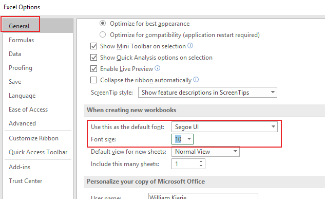
A theme is a set of formatting choices that includes theme colors, theme fonts and theme graphic formatting effects. Once saved, the theme is shared across other Office programs.

1. Set custom colours

To set our custom colours, we’ll go to Page Layout >>>Themes >>>Colors and click on Customize Colors…

custom theme colours in Excel

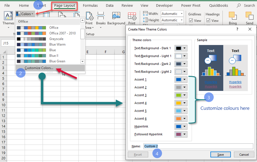
On the dialog box that appears (see right of the image above), change Accent 1 to Accent 6 colours which mainly influence the way your graphics will look.

Once happy with the colours, give this set of colours a name and click Save.

Next, you’ll set set your custom fonts.
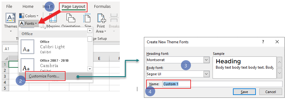
2. Set custom font

Go to Page Layout >>>Themes >>>Fonts and click on Customize Fonts…

You’ll get the dialog box below from which you can set the preferred font types for the headings and body text

custom theme fonts in Excel

We won’t go into selecting a preferred graphic formatting effect here as it is straight forward.

3. Save the theme with these custom colours and fonts

Once the theme colours and fonts are defined we now save the theme as follows:

Go to Page Layout >>>Themes >>>click on Save Current Theme…

custom theme in excel

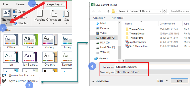
You’ll be prompted to enter the name of the theme. Ensure to retain the file type (or Save as type) option as Office theme (.thmx) and click save. The file location will be automatically chosen. Please do not change.

NOTE The saved theme will be available in other files so you can change the global feel of your Excel reports at a switch of the theme from Page Layout menu

3. Double click the fill handle -don't drag

This is often overlooked.

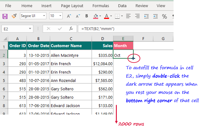
Funny enough, you’ll find most people manually dragging the fill handle to copy down a formula. So it takes almost if not a whole minute to get to the bottom of your data especially if it has many rows.

Not any longer

You just need to double-click the fill handle to copy the formula all the way down to the bottom of the table, so long as the adjacent column has data all the way to the last cell (i.e. if the adjacent column has a blank cell, then the formula will be auto-filled to that point)

double click fill handle for faster autofill

4. Improve your Excel files performance

Have you ever had an Excel file with minimal data but when you look at the file size it is 6, 7, 8 or more megabytes yet you expected it to be just a few kilobytes?

Bulk files can slow your pace in Excel

Well, here is the solution… this is what has worked for me

It is very common for people to highlight an entire column or row and apply highlight colour or borders or even conditional formatting.

This impacts on your file size.

>Select the columns/rows with extra formatting and either delete or from the Home tab, choose Clear Formats

To check what is the last used cell in your worksheet, press CTRL + End.

In some cases, you’ll notice that the actual area with data and the last used cell are different. Say, for instance, your data could be occupying up to cell J21 but when you press CTRL + END, you notice the last used cell is BB47760.

These extra cells with no data is what we’re referring to unused cells.

In this scenario, therefore:

  1. Select rows 22 to 47760 in this case, right click and choose delete
  2. Select columns K:BB, right click and choose delete
  3. Save the file and observe the change in file size

This has been one of my go to techniques when my files grow wildly large

By saving the file as .xlsb (binary mode), Excel compresses the file and also improves the speed of the file.

Save As .xlsb in Excel

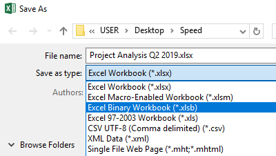
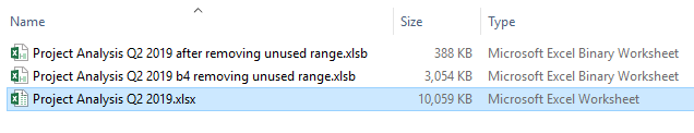
NOTICE that you may need to first remove unused range and then Save As in this .xlsb format to achieve greater compression.

See the screenshot below for results

.xlsb Excel format

Extra reading:

5. Implement Quick Access Toolbar (QAT)

Underline the word quick

QAT is a way to quickly access the features you commonly use, without having to move from one menu to the next.

To add a feature to the QAT, right-click the item in the ribbon and click “Add to Quick Access Toolbar.” I recommend adding these progressively from the Home tab, to Insert tab, and so on, in that order as you’ve formed a way of looking at these commands.

Excel Quick access toolbar

Once you’ve added the various commands, you can:

  1. Right click on the Ribbon and choose to display the QAT below the Ribbon
  2. Right click on the ribbon and choose to minimize/collapse the ribbon

You can do the same with other Office programs.

6. Master these key functions

These are my top pick that every analyst should know on the bare minimum, and are guaranteed to save you time:

  1. VLOOKUP
  2. PivotTables –Get started with this free online tutorial
  3. COUNTIFS
  4. Dollar sign ($)

7. Other Advanced Speed Boosters

Over time you’ll realize that achieving speed is a willingness to go an extra mile and explore more in Excel.

You’ll (where necessary) need to venture into:

  1. More advanced formulas and how to combine and nest them for flexible and dynamic analysis
  2. VBA / Macros -automate processes and potentially save over 90% of your manual tasks. Here is an illustration on how to combine multiple worksheets
  3. Power Query and Power Pivot -this is a way to automate data cleaning, modeling, analysis, and visualization without code. See an example here

Over to you

Am sure you have many other ways we can speed up our work as analysts in Excel. Please leave a tip in the comments below.

One request -help me empower many more to work faster in Excel by sharing this article in your preferred network below