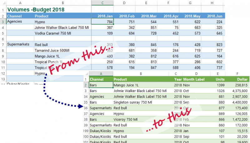
Most times when data is organized in Excel, it is done in a report format (cross tabulation) since it is easy to understand. Working with this format for further analysis can be an uphill task. It is therefore paramount for the analyst to be able to flatten the data into the conventional tabular layout. We shall look at how to use Power Query to unpivot data and do it in a scalable way.
You can download the file that goes with this blog to follow along.
If you prefer to watch the steps, here is the video:
Note that for the video and screen shots in this article we are using Excel 2013 but the steps will be very similar if you are using other Excel versions, with few exceptions of naming used.
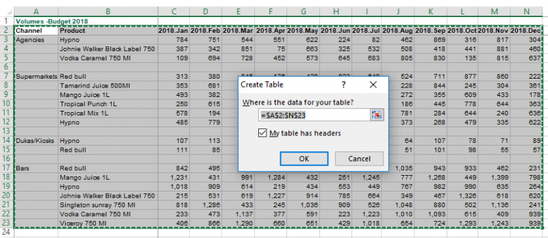
First, convert the data into a table
Select the range of data, in this case A2:N23
Press CTRL + T and ensure that “My table has headers” is ticked and press OK
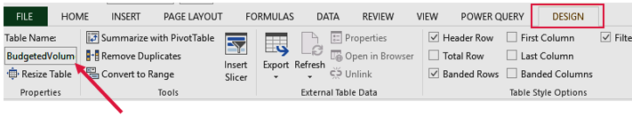
While within the data set, go to the contextual Design menu and rename the table to BudgetedVolumes (no spaces for a named range).
Load data to Power Query
Select any cell within the table
From the Power Query menu >>>click From Table/Range
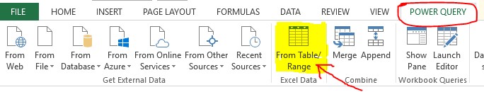
This will open up the Query Editor which we shall use to clean and shape our data to our liking.
Clean your data in Query Editor
We shall do a number of transformation as follows.
Eliminate blank rows
Our source data has a blank row at the end of each channel. We can use any of the columns apart from the Channel one to eliminate these blank rows. In this example, let us use the Product column.
- Click the filter handle against the Product column header
- Untick the null values to filter them out and press OK.
![]()
Next, we fill blank cells in the channel column
- Ensure you are within the Channel column.
- From the Query Editor >>>Transform menu >>>Fill >>>click the Down option
![]()
Use Power Query to Unpivot Data
At this point, we shall unpivot columns of data that hosts the budgeted units, that is, the 12 months columns will be collapsed into 2. One will have the period and the other column will have the units.
- Select the first two columns, that is channel and product columns.
- From the Transform menu >>>Unpivot Columns >>>Unpivot Other Columns
Alternatively, once you select the first two columns, you could right click and choose Unpivot Other Columns
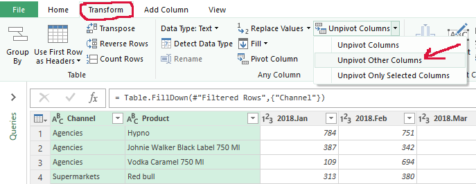
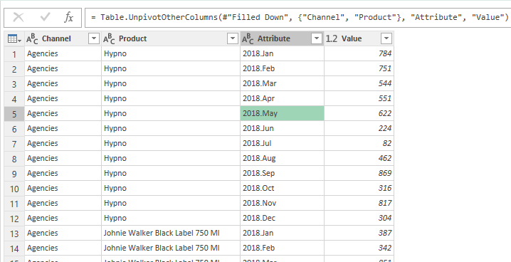
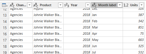
This action will yield the following:
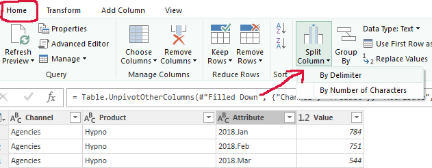
Split Column
Split the derived ‘Attribute’ column so that we have the year and month name as separate columns
- Select any value in the ‘Attribute’ column
- From Home menu >>>Split Column >>>By Delimiter
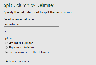
- From the dialog box below, choose Custom and type a period/full-stop as the delimiter and press OK to finish
- Finally, rename the columns appropriately. You should end up with the following at this juncture.
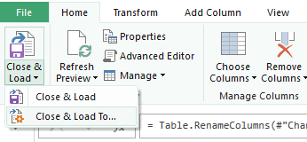
Load unpivoted data to Excel
Now that we have our data in the format that we wanted, we can load the data into an Excel worksheet and do further analysis.
From the Home tab >>>Close & Load >>>choose Close & Load To…
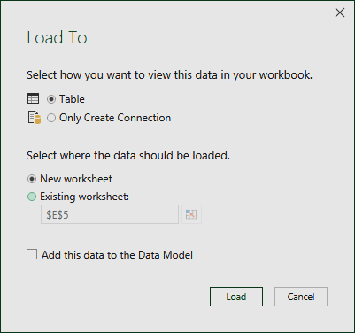
From the Load To window, ensure to tick Table and maintain New Worksheet as the destination. Don’t tick “Add this to the data model” unless you have Excel 2013/2016 and want to work with Power Pivot later.
Final thoughts
You could go ahead and load the price list table (see Excel file) and do a lookup of the product prices. This article doesn’t go into that.
If you would want to learn the steps involved, watch the video at the top of this page.
Please share this article on your preferred platform below and help us reach more working professionals with these time saving tips!

Discussion
Related
If you found some value from this, please explore our other articles below!
![Power BI DAX Measure [Crack the Challenge]](https://datacycleanalytics.com/wp-content/uploads/2019/05/DAX-Challenge-500x383.jpg?x66433)


